Quantification of dispersion of nanoparticles in polymer nanocomposites
While modification of polymers by addition of small amount of nanoparticles allows for extraordinary properties, the distribution and dispersion of the particles in the matrix dramatically affect the magnitude of changes. Factors affecting the dispersion include interfacial chemistry, matrix interactions and processing. For example, nanoparticles with poor interfacial interactions with the host matrix polymer tend to aggregate. Figure 1 shows such a poor dispersion of titania naoparticles in PMMA. Aggregation leads to reduced interphase volume, decreased stiffening, increased permeability and changes in the fracture behavior. However, it has been shown that certain degree of clustering can beneficially increase electrical percolation over ideally dispersed systems

Although dispersion controls these critical properties of nanocomposites, to date only limited studies have been performed to quantify the degree of dispersion and correlate the dispersion to mechanical and electrical property changes. In this work, we examine methods to quantify dispersion, coupling serial sectioning microscopy with analytical distribution functions. In addition, we will explore modeling as a nondestructive method to assess dispersion. This work includes examination of particle shape, size and orientation and their influence on aggregation. The influence of dispersion on macroscale nanocomposite properties will also be defined.
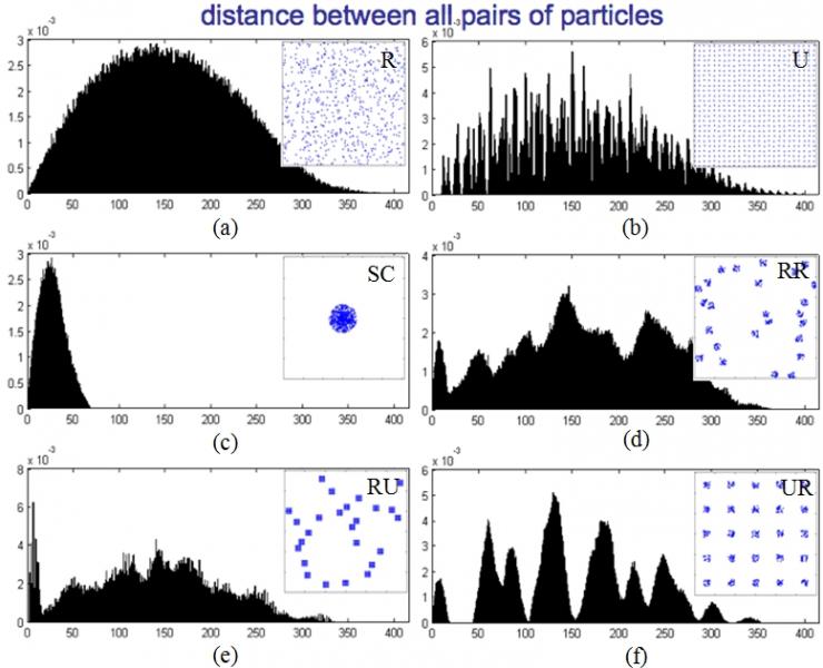
To simulate the dispersion of nanoparticles distributed on two dimensional surfaces of nanocomposites as seen in Figure 1, two dimensional models consisting of identical circles with various degrees of dispersion are generated. Figures 2a-2f show the frequency distribution of distances between all pairs of particles in random (R), uniform (U), single cluster (SC), randomly distributed random cluster (RR), randomly distributed uniform cluster (RU) and uniformly distributed random cluster (UR) models, respectively. While the histograms of the R and SC models indicate the normal distribution with different means and variances, the others show the discrete distribution corresponding to degree of uniformity.
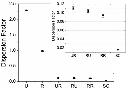
Subsequently, statistical distribution functions are applied to the models and the “dispersion factor” is determined for each model with different dispersion as shown in Figure 3. Whereas the dispersion factor of 1 and greater than 1 indicate the dispersion to be random and uniform, respectively, the clustering models have the factor less than 1. The factor expectedly approaches 0 for the SC model. This method of quantifying dispersion is sensitive enough to be able to distinguish the small differences among RR, RU and UR models. Work is ongoing to verify these results and correlate directly to experimental findings.